Svenesis Siril Scripts

A collection of Python scripts for Siril (astronomical image processing).

Author and links

Author: Sven Ramuschkat — www.svenesis.org
Repository: github.com/sramuschkat/Siril-Scripts

License

GPL-3.0-or-later

Official Siril Script Repository

✨ The following scripts are available in the official Siril Script Repository and can be installed directly from within Siril via Scripts → Get Scripts:

Svenesis Annotate Image
Svenesis Blink Comparator
Svenesis CosmicDepth 3D
Svenesis Gradient Analyzer
Svenesis Multiple Histogram Viewer

Scripts

Script	Description	Instructions	Siril Repo
Svenesis Annotate Image	Annotate plate-solved images with catalog objects, coordinate grids, and export as PNG/TIFF/JPEG.	Guide · DE	✨
Svenesis Blink Comparator	Animate a folder of FITS frames for rapid visual inspection and data-driven frame selection — statistics table, scatter plot, batch reject, file-based rejection workflow.	Guide · DE	✨
Svenesis CosmicDepth 3D	Render catalogued objects from a plate-solved image as a rotatable 3D scene — image plane with push-pin depth sticks, SIMBAD distances, stretched-log/linear/hybrid scaling, HTML/PNG/CSV export.	Guide · DE	✨
Svenesis CosmicView 3D	See where your astrophoto points in the universe — interactive 3D scene with the photo along its true line of sight, an auto-generated story card, a cinematic Journey flight from Earth to the target, and Story / Explorer view styles. Automatic Galactic / Cosmic mode, Planck18 cosmology.	Guide · DE	—
Svenesis LightCurve	Exoplanet transit photometry inside Siril, in the spirit of EXOTIC and HOPS: point it at a folder of sub-exposures and it measures the flux itself — follow-star re-centroiding, subpixel apertures, comparison stars kept by measured scatter — while Siril calibrates, registers (no resampling) and plate-solves. Limb-darkened transit fit with a calibrated significance floor, O−C against the published ephemeris, CSV/PNG/report and an AAVSO Exoplanet Watch file. Tested on EXOTIC's own sample data with matching results: Rp/R★ 0.1525 ± 0.0064 vs EXOTIC's published 0.1541 ± 0.0033 (0.2 σ), at the same scatter.	Guide · DE	—
Svenesis Gradient Analyzer	Analyze background gradients with heatmaps, diagnostics, and tool recommendations.	Guide · DE	✨
Svenesis ImageMono Train	Point it at one N.I.N.A. target folder and get finished colour: discovers the light frames per optical filter, calibrates them with whatever darks, flats and bias it finds, stacks a master for each (optionally only the ones the palette reads), aligns those channels onto a common grid, and combines them (LRGB · RGB · HaRGB · nine narrowband assignments · two weighted mixes) with background extraction and sensor-aware colour calibration (SPCC, including narrowband, with the sensor and filter names checked against Siril's own database). Writes a processing report and a step-by-step post-processing guide.	Guide · DE	—
Svenesis Multiple Histogram Viewer	View linear and stretched images with RGB histograms, 3D surface plots, and detailed statistics.	Guide · DE	✨
Svenesis Satellite Trail Cleaner	Per-frame satellite & aircraft trail detection and inpainting on FITS / XISF / TIFF / RAW subs — STScI's Median Radon Transform (`findsat_mrt`) detection, six inpaint methods with automatic per-frame recommendation, sky-noise matching, format-preserving round-trip, interactive line picker, parallel batch pipeline.	Guide · DE	—

Svenesis Annotate Image

File: Svenesis-AnnotateImage.py (v1.1.0) — Detailed Instructions · Deutsche Anleitung

✨ Available in the official Siril Script Repository.

Renders catalog annotations (deep-sky objects, named stars, coordinate grid, compass, info box) onto a plate-solved image and exports it as a shareable PNG, TIFF, or JPEG. All object data comes from live online VizieR and SIMBAD queries — no hardcoded or embedded catalogs. Parallel queries via ThreadPoolExecutor keep annotation fast even with multiple catalog sources. Inspired by PixInsight's AnnotateImage script. Unlike Siril's built-in overlay annotations, this script burns the annotations into an exportable image — ready to post on social media, forums, or include in observation reports.

Screenshots

Main window: catalog annotations with object type filtering, coordinate grid, compass rose, info box, and color-coded legend. Preview tab shows the annotated result.

Features

Object selection by type

Instead of choosing catalogs, you select which types of objects to annotate. All online catalog sources are queried in parallel — objects are filtered by your type selection:

Color	Type	Examples
Gold	Galaxies	M31, M51, M81, NGC 4565, Centaurus A
Red	Emission Nebulae	Orion, Lagoon, Eagle, Rosette, Carina
Light red	Reflection Nebulae	M78, Witch Head, Iris, Rho Ophiuchi
Green	Planetary Nebulae	Ring (M57), Dumbbell (M27), Helix, Owl
Light blue	Open Clusters	Pleiades (M45), Double Cluster, Wild Duck
Orange	Globular Clusters	M13, Omega Centauri, 47 Tucanae
Magenta	Supernova Remnants	Crab (M1), Veil Nebula, Simeis 147
Grey	Dark Nebulae	Horsehead (B33), Pipe, Snake, Coalsack
Red-pink	HII Regions	Heart, Soul, Barnard's Loop, Cave Nebula
White	Named Stars	~275 IAU-named stars to mag ~5.5
Pale blue	Asterisms	Coathanger, Kemble's Cascade
Violet	Quasars	QSOs and AGN from SIMBAD

Select All / Deselect All buttons for quick toggling.

Online catalog sources

VizieR VII/118 (NGC 2000.0) — NGC, IC, and Messier objects
VizieR VII/20 (Sharpless 1959) — HII regions
VizieR VII/220A (Barnard 1927) — Dark nebulae
VizieR V/50 (Yale BSC) — Named bright stars
SIMBAD — Supplementary objects (UGC, Abell, Arp, Hickson, Markarian, vdB, PGC, MCG, etc.) plus common name resolution

All data from live online queries — no hardcoded object data. Survey catalog junk (SDSS, 2MASS, GPM, Gaia, etc.) is automatically filtered out. Requires astroquery package and internet connection.

Annotation overlays

Leader lines: Thin connecting lines from each label to its object marker — essential in crowded fields to see which label belongs to which object.
Color legend: Auto-generated legend box (bottom-left) showing only the object types present in the current annotation.
Coordinate grid: RA/DEC grid with auto-spaced lines and labeled coordinates.
Info box: Semi-transparent box (top-left) with center RA/DEC, field of view, pixel scale, rotation, and object count.
Compass rose: North/East direction arrows derived from WCS.

Display options

Configurable font size, marker size, and magnitude limit
Object size rendered as scaled ellipses (from catalog angular size)
Common names display (e.g. "M31 (Andromeda Galaxy)")
Optional magnitude and type labels
Color coding by object type (configurable)
Label collision avoidance (32-candidate greedy algorithm with spatial grid scoring)

Output

Formats: PNG (recommended), TIFF, JPEG
DPI: 72–300 (150 default for screens, 300 for print)
Auto-timestamped filenames prevent overwriting
Preview tab shows the result immediately after annotation
Open output folder / Open image buttons for quick access

WCS detection

Robust plate-solve detection with 6 fallback strategies:

FITS header as dict (primary — same approach as Galaxy_Annotations.py)
FITS header as string (astropy parsing)
Keywords pltsolvd / wcsdata flag check
pix2radec sampling to build WCS from Siril's coordinate transform
pix2radec probe without plate-solve flag
FITS file on disk

Coordinate transforms use siril.radec2pix() for maximum compatibility.

Other features

Persistent settings: All checkboxes, sliders, and options saved between sessions via QSettings
Keyboard shortcut: F5 = Annotate
Progress bar with status feedback during annotation
Log tab with detailed diagnostic output
Dark-themed PyQt6 GUI matching Gradient Analyzer style
Buy me a Coffee support dialog
Parallel catalog queries via ThreadPoolExecutor
Thread-safe siril coordinate access
Large mosaic support (display downscaling, DPI capping, memory management)
Common names from SIMBAD with catalog-name filtering
Two-column checkbox layout for all option groups

Requirements

Siril 1.4+ with Python script support
sirilpy (bundled with Siril)
numpy, PyQt6, matplotlib, astropy, astroquery (installed automatically via s.ensure_installed)

Usage

Load an image in Siril and plate-solve it (Tools → Astrometry → Image Plate Solver).
Run Svenesis Annotate Image from Siril: Processing → Scripts (or your Scripts menu).
Select which object types to annotate using the color-coded checkboxes.
Adjust font size, marker size, magnitude limit, and extras (grid, info box, compass, legend, leader lines).
Click Annotate Image (or press F5).
Review the result in the Preview tab. Use Open Annotated Image to view it full-size.

Svenesis Blink Comparator

File: Svenesis-BlinkComparator.py (v1.2.8) — Detailed Instructions · Deutsche Anleitung

✨ Available in the official Siril Script Repository.

Picks a folder of FITS frames, builds a temporary svenesis_blink sequence in Siril, and animates it as a blink animation for rapid visual inspection and data-driven frame selection. Comparable to PixInsight's Blink + SubframeSelector — identify satellite trails, clouds, tracking errors, focus drift, and bad frames, then reject them with a single click. Rejections are collected locally and, on close, written as rejected_frames.txt next to your files (with the physical FITS moved into a rejected/ subfolder). Your original frames are never modified.

Screenshots

Main window: viewer with frame info overlay, sortable statistics table, statistics graph with running average, scatter plot, thumbnail filmstrip, batch selection, and approval expressions.

Features

Folder-based workflow

At startup the script always prompts for a folder of FITS files (recurses one level) and builds a temporary svenesis_blink FITSEQ sequence via convert -fitseq (and optional register -2pass for star stats).
The temp sequence is automatically cleaned up when you close the window.
Rejections write a plain-text rejected_frames.txt audit file and move rejected FITS into a rejected/ subfolder — reversible by simply dragging the files back.
Completely non-destructive: original frames are never overwritten.

Animated playback

Configurable speed (1–30 FPS) with loop option and Play/Pause (Space key)
Frame navigation: First, Previous, Next, Last buttons + draggable color-coded slider
Only included filter (checkbox) to skip rejected frames during playback
Color-coded slider: Red tick marks at excluded frame positions for instant overview

Two display modes

Normal: Single-frame autostretched view. Default. Used for visual inspection, satellite/cloud hunting (play at 3–5 FPS — changing pixels jump out to the eye), and focus/tracking review.
Side by Side (vs. reference): Current frame on left, reference (first frame) on right, synchronized zoom/pan. For direct A/B comparison.

Autostretch presets

Conservative — darker background, preserves dim detail.
Default — PixInsight-style STF (shadows_clip = -2.8, target median = 0.25).
Aggressive — brighter, higher contrast.
Linear — no stretch, raw data clipped to 0–255.
Switching presets invalidates caches and re-renders; the choice is persisted across sessions via QSettings. Autostretch is always globally linked — every frame uses the same median/MAD so brightness differences (clouds, haze) stay visible.

Statistics table (sortable)

All frames listed with Weight, FWHM, Roundness, Background, Stars, Date, Status
Click any column header to sort — sort by FWHM to instantly find the worst frames
Click a row to jump to that frame in the viewer
Multi-select (Ctrl+click, Shift+click) → right-click → "Reject selected"

Composite quality weight

Each frame gets a normalized quality score (0–1) based on FWHM (lower=better), roundness (higher=better), background (lower=better), and star count (more=better)
Sort by Weight to see best and worst frames at a glance

Statistics graph

FWHM, Background, Roundness plotted as line charts across all frames
Running average (7-frame moving average) for trend detection
Excluded frames shown as red dots, current frame as white dashed line
Instantly reveals focus drift, clouds rolling in, or tracking degradation over time

Scatter plot

2D scatter of any two metrics (FWHM vs Roundness, FWHM vs Background, etc.)
Outlier frames immediately visible as dots far from the cluster
Click a dot to jump to that frame
Axis-normalized click detection (both axes contribute equally to nearest-point selection)

Frame selection

Manual marking: G = include, B = exclude (with auto-advance to next frame)
Batch reject by threshold: Reject all frames where FWHM > 4.5 (or any metric/operator/value combination) with live preview count
Reject worst N%: Reject the worst 10% by FWHM, Background, Roundness, or Weight
Approval expressions: Multi-criteria AND filter (e.g., FWHM < 4.5 AND Roundness > 0.7 AND Stars > 50) — rejects frames that fail any condition
Multi-select in table: Ctrl+click or Shift+click rows, right-click → "Reject selected"
Reset All Rejections: One-click button to mark every frame as Included again (baseline + pending) — useful when you want to start the selection over
Undo (Ctrl+Z): Single undo for individual marks, grouped undo for batch operations (one Ctrl+Z undoes the entire batch)
Pending changes shown in the left panel — only committed on close via "Apply Rejections && Close"

Thumbnail filmstrip

Horizontal scrollable strip with color-coded borders: green = included, red = excluded, blue = current
Click any thumbnail to jump to that frame
Lazy loading: Thumbnails loaded on demand as you scroll
Adjustable size: Slider in the viewer toolbar (40–160 px)
Thumbnail cache reuses the main frame cache's already-stretched display data to avoid redundant disk I/O

Zoom & pan

Scroll wheel zoom (0.1x–20x), right-click drag pan
Fit-in-Window button (or Z) to return to full-frame view
Live zoom-percentage readout that updates during scroll-wheel zoom

Frame info overlay

Frame number, FWHM, roundness, and quality weight burned into the image corner during playback
Toggleable via the Overlay checkbox in the viewer toolbar

Export

Statistics CSV (full table with all metrics + inclusion status)
Animated GIF of the blink animation (included frames, scaled to 480 px)
Copy to clipboard (Ctrl+C) — captures the composite canvas (side-by-side layout + overlay, not just the raw pixmap)

Other features

A/B frame toggle (T key): Pin the current frame, press T to toggle between the pinned frame and the current one
Session summary on close: Frames viewed, excluded count, mean/best/worst FWHM
Persistent settings: FPS, loop, auto-advance, overlay, autostretch preset, thumbnail size, display mode, table sort column, graph metric visibility
Post-mark refresh debouncing: Rapid G/B marking collapses slider-exclusions repaint, scatter-plot rebuild, and statistics-graph rebuild into a single coalesced 150 ms refresh — hotkeys stay snappy even on 2000-frame sequences
Dark-themed PyQt6 GUI matching Gradient Analyzer style
Buy me a Coffee support dialog

Keyboard shortcuts

Key	Action
`Space`	Play / Pause
`←` / `→`	Previous / Next frame
`Home` / `End`	First / Last frame
`G`	Mark frame as good (include)
`B`	Mark frame as bad (exclude)
`Z`	Fit-in-window (reset zoom)
`T`	Pin / toggle A/B frame comparison
`Ctrl+Z`	Undo last marking (single or batch)
`Ctrl+C`	Copy current frame to clipboard
`1`–`9`	Set playback speed (FPS)
`+` / `-`	Speed up / slow down
`Esc`	Close (with "apply / discard / cancel" prompt if changes are pending)

1–9 are handled through keyPressEvent instead of QShortcut, so digits typed into focused spinboxes/line-edits still reach the widget for multi-digit entry.

Requirements

Siril 1.4+ with Python script support
sirilpy (bundled with Siril)
numpy, PyQt6, matplotlib (installed automatically via s.ensure_installed)
Optional: Pillow (for GIF export)

Usage

Run Svenesis Blink Comparator from Siril: Processing → Scripts (or your Scripts menu).
A folder picker opens — select a folder containing your FITS frames (registered or unregistered). The script builds a temporary svenesis_blink sequence and loads all frame statistics.
If the FWHM / Roundness / Stars columns are empty, click the yellow "Run Star Detection" banner (runs register -2pass — non-destructive).
Use the Statistics Table tab to sort by FWHM and identify bad frames, or play the sequence at 3–5 FPS in Normal mode and mark frames with B (auto-advances).
Use Batch Selection (threshold / worst N%) or Approval Expression for bulk rejection.
Review in the Statistics Graph and Scatter Plot tabs to verify your selection.
Click Apply Rejections && Close — the script writes rejected_frames.txt next to your FITS files and moves rejected frames into a rejected/ subfolder, then closes. Drag files out of rejected/ to undo a decision after the fact.

Changes Since v1.2.3

The last officially published release was v1.2.3. Summary of what has changed since then (see the script's CHANGELOG block for one-line bullets per release):

v1.2.4 — Folder-only workflow. The script now always prompts for a folder of FITS files and builds its own temp sequence. Rejected frames move to a rejected/ subfolder alongside a rejected_frames.txt audit file. Added an autostretch preset dropdown (Conservative / Default / Aggressive / Linear). Removed the ROI feature, the per-frame histogram widget, and the "use currently loaded sequence" path.
v1.2.5 — Simplified display modes. Removed the Difference display mode and the D shortcut (playing at 3–5 FPS in Normal mode catches the same artifacts). Removed the Linked-stretch toggle — globally-linked autostretch is now the only mode.
v1.2.6 — Performance pass. Thumbnails reuse the main frame cache's already-stretched image, mtf() runs in-place, RGB autostretch is a single pass, and preload pacing follows FPS.
v1.2.7 — Marking responsiveness. Rapid G/B marking coalesces slider / scatter / graph refreshes through a single 150 ms timer; filmstrip and table skip no-op styling work.
v1.2.8 — Cross-platform polish & stability. UTF-8 for rejected_frames.txt and CSV export (fixes Windows non-ASCII paths). 1–9 FPS presets moved to keyPressEvent so focused spinboxes accept digits natively. Folder paths with spaces are now quoted in Siril commands. Apply moves files first, then writes an audit list of only what actually moved. Star detection rebinds caches/stats and advances the progress bar through post-register phases. View-state (filter, display mode, graph metrics, scatter axes) now persists across sessions.

Svenesis CosmicDepth 3D

File: Svenesis-CosmicDepth3D.py (v1.0.1) — Detailed Instructions · Deutsche Anleitung

✨ Available in the official Siril Script Repository.

Takes every catalogued object in your plate-solved image, resolves their distances from SIMBAD (mesDistance, redshift/Hubble law, type-median fallback) and renders them as a rotatable 3D scene. Your image sits as a flat "window" at the front; each object hovers at its actual distance behind the window on a push-pin depth stick that lands on the exact pixel of the feature in the sky plane. A foreground nebula at 1,344 ly and a background galaxy at 30 million ly finally look like what they are.

Screenshots

Features

3D scene layout

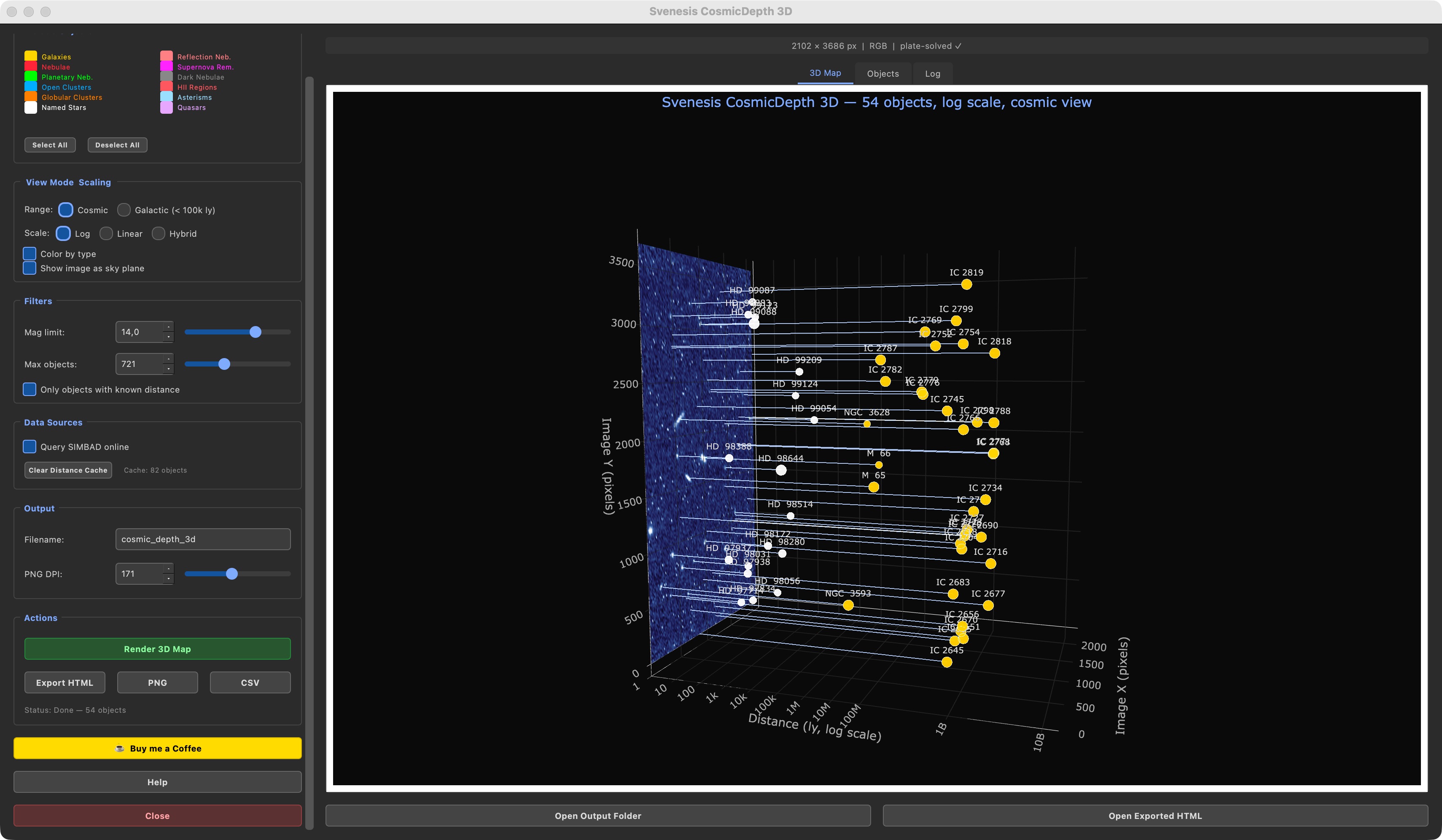
Image plane rendered as a flat, non-transparent rectangle at the front of the scene, with the same orientation as the Siril image (FITS row 0 at the bottom, pixel-X mirrored so the default camera angle reads left/right like Siril).
Depth sticks from each object marker straight back to its exact image pixel — the "push-pin through a window" view.
Embedded rotatable view via QWebEngineView + Plotly: drag to rotate, scroll to zoom, hover any marker for distance, uncertainty and source. Falls back to a static PNG plus opening the interactive HTML in the browser if WebEngine is unavailable.
Viewer-from-Earth perspective — X = depth (scaled ly), Y = pixel-X (mirrored), Z = pixel-Y (direct). Axis proportions follow the image aspect so the scene box matches the frame.

Scaling & view ranges

Stretched-log (default) — piecewise-log distance axis: each decade below 100 M ly takes 1 unit, each decade beyond takes 3 units, so the far-galaxy tail gets ~3× more room on screen than a plain log would give it. Tick labels read in real light-years (1, 10, 100, 1k, …, 100M, 1B, 10B). Recommended for most fields.
Linear — true proportional distances. Useful for star-only fields inside the Milky Way (galaxies disappear to the horizon).
Hybrid — linear up to 10,000 ly, log beyond. Realistic solar-neighbourhood spacing with extragalactic context preserved.
View ranges: Cosmic (everything) or Galactic (< 100,000 ly, i.e. inside the Milky Way only).

Distance resolution

Priority chain: local JSON cache (90-day TTL) → SIMBAD mesDistance table → redshift × Hubble law (z < 0.5) → type-based median fallback (clearly labelled as Type median).
Distance cache in ~/.config/svenesis/cosmic_depth_cache.json — a second render of the same field is near-instant.
Clear Distance Cache button to force a full re-query (useful after SIMBAD updates).

Object selection by type

Same colour-coded type system as Annotate Image:

Color	Type	Typical distance range
Gold	Galaxies	2 Mly – billions of ly
Red	Emission Nebulae	500 – 10,000 ly
Light red	Reflection Nebulae	400 – 1,500 ly
Green	Planetary Nebulae	1,000 – 10,000 ly
Light blue	Open Clusters	400 – 15,000 ly
Orange	Globular Clusters	10,000 – 100,000 ly
Magenta	Supernova Remnants	500 – 30,000 ly
Grey	Dark Nebulae	400 – 2,000 ly
White	Named Stars	10 – 5,000 ly
Red-pink	HII Regions	1,000 – 30,000 ly
Pale blue	Asterisms	various
Violet	Quasars	billions of ly

Performance

Parallel SIMBAD tiling — wide fields are split into ≤ 0.75° tiles and queried with up to 8 concurrent TAP requests, with live per-tile progress feedback in the status bar.
Cached plotly.min.js — written once to your temp directory and referenced from each render, so refreshes reload only the (small) scene data rather than the ~3.5 MB Plotly bundle.
Opt-in WebEngine repair — if the installed PyQt6-WebEngine wheel doesn't match Siril's bundled PyQt6 Qt version (symptom: Symbol not found: _qt_version_tag_6_XX), the embedded view shows a red banner with a "Repair WebEngine…" button. Clicking it opens a dialog with the exact pip command, live stdout/stderr, and a Retry button. The repair is skipped automatically on PEP 668 / externally-managed Python interpreters; no silent force-reinstalls.

UI

3D Map tab — embedded rotatable Plotly scene (or static PNG fallback with a banner if WebEngine is unavailable).
Objects tab — sortable QTableWidget with Name, Type, Mag, Distance (ly), ± uncertainty, Source. Click any column header to sort numerically; column widths and sort order persist between sessions.
Log tab — detailed diagnostic output (SIMBAD tile counts, cache hit rate, fallback reasons).
Help dialog — 4 tabs (Getting Started, Object Types, Scaling & Display, Exports & Performance) matching the Annotate Image help style.
Dark-themed PyQt6 GUI consistent with the rest of the suite.

Export

HTML — standalone, fully interactive Plotly scene (shareable, opens in any browser).
PNG — high-resolution static export via Plotly + kaleido, captured from your current 3D camera angle and zoom so the saved image matches what you see on screen (including the stretched-log axis with ly labels). Falls back to a matplotlib snapshot if kaleido isn't installed.
CSV — full object table: name, type, RA/Dec, magnitude, size, distance, uncertainty, source, confidence, image pixel (x, y).

All exports are written to Siril's working directory with a timestamp appended to the base filename.

Requirements

Siril 1.4+ with Python script support
sirilpy (bundled with Siril)
numpy, PyQt6, matplotlib, astropy, astroquery, plotly, kaleido (installed automatically via s.ensure_installed)
PyQt6-WebEngine — probed at startup; if missing or ABI-mismatched the script offers an explicit in-app repair dialog and falls back to a static view + browser HTML in the meantime
Internet connection for the initial SIMBAD queries (subsequent renders use the local distance cache)

Usage

Load an image in Siril and plate-solve it (Tools → Astrometry → Image Plate Solver).
Run Svenesis CosmicDepth 3D from Siril: Processing → Scripts (or your Scripts menu).
Select which object types to include (left-panel checkboxes), set the magnitude limit, and pick a scaling mode and view range.
Click Render 3D Map (or press F5).
Drag in the scene to rotate, scroll to zoom, hover markers for details. Toggle Show image as sky plane to switch between the pixel-mapped "window" layout and a pure abstract 3D map.
Review the Objects tab for the full distance table; use Export HTML / PNG / CSV for sharing or archiving. The PNG export captures your current camera angle, so rotate first to the view you want.

Svenesis CosmicView 3D

File: Svenesis-CosmicView3D.py (v1.0.0) — Detailed Instructions · Deutsche Anleitung

⚠️ Public preview — not yet submitted to the official Siril Script Repository.

Reads the current plate-solved image from Siril, identifies the main astronomical object via SIMBAD, and renders where your photo points in the universe as an interactive 3D model — Earth in the Orion Arm, the astrophoto as a textured rectangle along the exact line of sight, and the target's distance made tangible through a story card, scale rings, and a cinematic Journey flight from Earth to the target. CosmicView 3D answers a question that no other tool answers: "My photo is not just anywhere — it is a window into one specific direction of the universe. Where exactly?"

CosmicView vs. CosmicDepth: the sibling script CosmicDepth 3D shows the depth of everything inside one photo (each catalogued object on its own push-pin at its true distance). CosmicView 3D zooms out to show where that whole photo sits in the galaxy and the universe, seen from Earth.

Screenshots

Main view: 5-arm Milky Way with galactic disk stars, Earth in the Orion Arm, and the plate-solved astrophoto rendered as a textured rectangle pointing in its actual viewing direction. Drag to rotate, scroll to zoom.

Features

The human experience

Opening pull-back — the first render of a target starts at Earth's point of view (the sky as you saw it), holds a beat, then pulls back to reveal the whole map. Plays once per target; can be disabled in Scene Elements.
🚀 Journey mode — a ~11-second cinematic camera flight from Earth along your photo's line of sight out to the target, with a live HUD counter ("38.7 Mly from Earth — the light in your photo passed this point 38.7 million years ago") and waypoint callouts (leaving the Local Bubble, leaving the Milky Way, passing Andromeda, …). Also available via the J key — including in exported HTML.
Story card — an auto-generated narrative shown over the 3D view and in the Info tab: where you pointed, how old the light is (anchored to Earth history: "…just after the dinosaurs died out"), which spiral arm the target sits in, and a dinner-plate scale analogy. Included in CSV exports and baked into PNG exports as a caption.
Story / Explorer view styles — Story (default) keeps only the narrative thread: Earth, viewing ray, photo, target, galaxy structure, distance rings. Explorer adds every reference overlay: landmark catalogs, galaxy-cluster halos, the CMB observable-universe boundary, Local Bubble / Local Group context spheres.

Two automatic view modes

Galactic mode (object distance < 150,000 ly): 1 unit = 1,000 ly, linear. Spiral arms (with camera-distance fade), disk stars, bulge, Sgr A*, Earth reticle with orbital-motion arrow, GC-centred and Earth-centred distance rings, constellation stick figure at the target's depth, Local Bubble for nearby targets, and a curated in-galaxy landmark catalog (Pleiades, M42, M13, Veil, Carina, …).
Cosmic mode (≥ 150,000 ly): 1 unit = 100,000 ly, log-compressed beyond 1 Mly (boundary marked). Neighbour galaxies with hover-rich descriptions, galaxy-cluster halos (Virgo, Coma, Perseus, Shapley, …), a cosmic landmark catalog, and the CMB last-scattering surface at 13.8 Gly as a wireframe globe.
Mode is selected automatically from the resolved distance and SIMBAD type; override any time.

Distance & cosmology

Priority chain: local JSON cache (90-day TTL) → SIMBAD mesDistance table → redshift → Planck18 light-travel distance (astropy.cosmology; H₀ ≈ 67.4) → parallax where reliable → type-median fallback (clearly labelled).
Parallax sanity check — SIMBAD's noise parallaxes on extragalactic objects are rejected when a significant redshift disagrees by >100×.
Distance-metric toggle — view the cosmic scene in light-travel, comoving, or angular-diameter distance; the 3D positions physically reorganise and the HUD always states the active metric.
Distance rings drawn flat (radar-style) with depth fading; the one ring nearest your target's distance becomes a spherical shell — "your photo sits at this depth."
Offline-friendly — cone-search results are cached 7 days; re-renders of known targets need no network. A SIMBAD health probe shortens timeouts during outages, and all network calls run off the UI thread.

Photo placement in 3D space

Plate-solved WCS ingestion with the same 6-strategy WCS detection used by CosmicDepth 3D.
Photo as a textured rectangle: four image corners converted RA/Dec → galactic, FITS auto-stretched and applied as the surface texture (resolution configurable; auto-capped in cosmic mode for performance).
Viewing ray from Earth to the photo centre — the line literally shows where your telescope pointed.
Background depth sticks — SIMBAD objects behind your target are drawn at their true distance and connected radially to their exact pixel position on the photo.

Interactive 3D rendering

Plotly-in-QWebEngineView: drag-to-rotate, scroll-to-zoom, hover-for-details, camera presets (Earth POV / Top / Side / Iso), trackball + zoom pad, auto-rotate, rescue keys (R / Home / Esc), double-click a spiral-arm legend entry to fly to that arm.
Live scale ruler and context-aware zoom hints that track the camera in real time.
Matplotlib 3D fallback if PyQt6-WebEngine is unavailable.
Dark-themed PyQt6 GUI; view style, distance metric, and all scene toggles persist via QSettings.

Target picker

A target picker dialog lists all SIMBAD cone-search candidates with type, magnitude, distance (with source hint: z / π / type), size in photo, and offset — so you choose the actual photographic subject. Candidates can be exported as JSON.

Export

HTML — standalone, fully interactive Plotly scene including the Journey (J key) and story toast.
PNG — high-resolution snapshot of the current camera angle, with the story text appended as a caption band.
CSV — scene metadata including redshift, lookback time, distance metric, cosmology, arm membership, the story text, and photo-corner coordinates.

Requirements

Siril 1.4+ with Python script support
sirilpy (bundled with Siril)
numpy, PyQt6, matplotlib, astropy, astroquery, plotly, Pillow, kaleido, requests (installed automatically via s.ensure_installed)
PyQt6-WebEngine — probed at startup; if missing or ABI-mismatched the script falls back to a static matplotlib view
Internet connection for the initial SIMBAD queries (subsequent renders use the local caches)

Usage

Load an image in Siril and plate-solve it (Tools → Astrometry → Image Plate Solver).
Run Svenesis CosmicView 3D from Siril: Processing → Scripts (or your Scripts menu).
Confirm (or change) the identified target in the picker dialog.
Watch the opening pull-back reveal where your photo sits; read the story card.
Press 🚀 Journey (or J) to fly the light path from Earth to your target.
Switch Story ↔ Explorer in Scene Elements for the clean narrative view or the full reference map.
Use Export HTML / PNG / CSV to share or archive the view.

Development

tests/test_cosmicview.py (pure-function tests) and tests/js_harness.mjs (embedded-JS camera/overlay tests) run with plain python3 / node — no Siril required.

Svenesis LightCurve

File: Svenesis-LightCurve.py (v1.0.3) — Detailed Instructions · Deutsche Anleitung

Exoplanet transit photometry inside Siril, in the spirit of EXOTIC (NASA's Exoplanet Watch pipeline) and HOPS — and tested against EXOTIC on its own sample data, with matching results. Point it at the folder holding one night's sub-exposures of an exoplanet host star. It measures how that star's brightness changed relative to other stars in the same field, removes the systematic trends it can account for, fits a transit — and tells you whether the dip is real.

Who does what

Siril does what it is demonstrably good at: staging, calibration, two-pass registration, star detection, the plate solve and per-frame quality.

The script measures the flux itself, the way EXOTIC and HOPS do: every star re-centroided per frame from its registration-predicted position (the "follow star" Siril's light_curve lacks), subpixel circular apertures against a sigma-clipped sky annulus, the aperture chosen by point-to-point noise, comparison stars kept or dropped by their measured scatter, errors from the CCD equation with every term measured. Measured on the same drifting 142-frame run: this engine keeps 140 points at 6.3 mmag where Siril's light_curve kept 67 — and light_curve remains intact as the loud fallback. The script also does the parts nobody's pixels decide: which star is the target, how to remove the airmass ramp without eating the transit depth — and whether to claim anything at all.

Validated against EXOTIC on its own sample data (HAT-P-32 b, 142 frames): Rp/R★ = 0.1525 ± 0.0064 against EXOTIC's published 0.1541 ± 0.0033 — 0.2 σ apart — at the same residual scatter (0.58 % vs 0.55 %). Both depth conventions are reported and labelled: the limb-darkened central depth the fit measures, and the (Rp/R★)² that EXOTIC, HOPS and AstroImageJ quote (~20 % shallower on a solar-type star — compare that one with theirs and with the archive).

Why not just Siril's own light-curve tool? That workflow produces a light curve; this script produces a measurement — follow-star re-centroiding, drift handling and comp screening that light_curve lacks (140 of 142 points where it kept 67 on the same run), plus the analysis the native tool ends before: BJD_TDB, a simultaneous limb-darkened fit, calibrated significance, O−C and the AAVSO file. The full comparison is in the manual's FAQ.

Calibration finds its own frames. Point at the subs — or at any folder above them, the scan is recursive and sorts lights from calibration frames by header — and, once, at the folder where your reusable darks live; the flats are found beside the lights in the N.I.N.A. LIGHT/FLAT layout, grouped by exposure/gain/temperature/binning/size/camera, stacked into masters and cached for the next run. The pixel work is Siril's calibrate — there is no bias/dark/flat arithmetic in the script, for the same reason there is no photometry in it. What gets refused is said out loud, because a master that was found and rejected leaves a run that looks exactly like one where no master existed: a dark at the wrong exposure is named with what the mismatch would have done, darks are split by temperature and bias is not, and bias is never applied together with a dark — the dark already carries the offset, so it corrects the flats instead.

Taken from EXOTIC, measured before and after. The aperture is now chosen — six radii from 0.75 to 2.5 FWHM, each photometered, least scatter wins — instead of whatever -autoring derived. Comparison stars are photometered against each other and dropped on their own variability. And there is spike rejection, which mattered more than it looks: one 100 mmag outlier on a real 12 mmag transit took the significance from 12.1σ to 3.2σ, under the detection floor, so a measured transit read as not claimed. A robust post-fit scatter recovers 6.9σ of that and removing the point recovers the rest. The run also writes an AAVSO Exoplanet Watch file — refused unless the times are BJD_TDB.

Three decisions worth knowing about

Registration without resampling. register -2pass computes registration data and stops. seqapplyreg would interpolate every pixel, and interpolation correlates neighbouring noise and moves flux inside the aperture. Siril's photometry follows the stars through the registration data instead, so the aperture lands on the star while the pixels stay exactly as the sensor recorded them.

The airmass detrend does not eat the depth. A plain fit through every point absorbs part of the transit whenever the dip correlates with the ramp — the standard evening-target case. The baseline is fitted with a one-sided least-trimmed pass, then re-fitted directly on the points outside the transit window. Measured on synthetic runs with a known 30 mmag/airmass ramp: a plain fit recovers the slope 6–11 % low; this lands within 1 % up to 50 % duty cycle, and within 3 % at 75 % where the blind pass alone is no better than the plain fit.

The significance test is two-sided. A real transit returns to the baseline it left; a trend does not. Pooling both sides into one out-of-transit mean loses that: on a monotonic ramp with no transit in it — uncorrected extinction, a drifting cloud, focus creep — the pooled contrast reaches +25σ. Comparing each side separately and taking the weaker returns −10σ on the same data. The floor below which nothing is claimed is calibrated, not chosen: the significance is the best of ~40 000 grid nodes, so it is not a Gaussian σ. Measured over 1200 transit-free noise runs through that same search, a 3σ floor lets one run in ten through — where the label is read as one in 750 — while 4.5σ gives 0.25 % and still detects 89 % at 6 mmag and 100 % at 8. The table has been re-measured three times — a finer search, a robust scatter, and a limb-darkened model fitted simultaneously with the systematics: a calibration is only valid for the search, the statistic and the model it was measured on. The measured rate is printed next to every result. A transit clipped by the start or end of the run returns zero, because without baseline on both sides the question cannot be answered.

Output

lightcurve/lightcurve.csv (JD, raw, centred, detrended, error, airmass), the plot as PNG, a plain-text report with the comparison stars, every rejection and its reason, the method, and the result — and, when the times are BJD_TDB, an AAVSO_exoplanet.txt in Exoplanet Watch's format with T0 ± error, both depth conventions, Rp/R★ ± error and duration in the header.

Tests

tests/test_lightcurve_helpers.py runs with plain python3 — no Siril required. Over 450 checks against input with a known answer: the J2000 epoch, sec z, synthetic transits of stated depths recovered by the full photometry engine and the full fit, twelve pure-noise runs that must not be claimed, the monotonic ramp that the two-sided test exists for, error bars calibrated against 24 independent synthetic nights, and the limb-darkened depth conventions round-tripped through the same model the fit uses.

Svenesis Gradient Analyzer

File: Svenesis-GradientAnalyzer.py (v1.8.4) — Detailed Instructions · Deutsche Anleitung

✨ Available in the official Siril Script Repository.

Reads the current image from Siril, divides it into a configurable grid of tiles, computes sigma-clipped median background levels per tile, and renders a color-coded heatmap. It helps you assess background gradients (e.g. from light pollution), decide whether background extraction is needed, and choose the right tool and parameters for the job.

Screenshots

Main window: heatmap with sample point guidance, 3D surface view, gradient strength gauge, and quadrant analysis. Nine visualization tabs with context-sensitive descriptions.

Features

Beginner-friendly UI

"What is a gradient?" introduction: Getting Started tab explains gradients with a visual analogy and common causes (light pollution, vignetting, sensor artifacts) before any technical details.
Beginner Glossary: Technical Reference tab includes 25+ plain-language definitions (gradient, flat/dark/bias frames, linear/stretched, polynomial degree, R², FWHM, SNR, tool names).
Self-explaining action plan: Each step explains what the term means, why it matters, and how to do it in Siril (including menu paths and Console instructions).
Tiered Analysis Results: Summary & Actions tab with color-coded verdict, plain-English explanation, and prioritized action plan. Detailed Metrics tab with inline jargon explanations. Before/After delta tab when re-analyzing.
Tiered Recommendations: Quick Guide tab with styled, categorized suggestions (critical issues, tools, workflow). Full Details tab with raw diagnostic output.
Organized Help dialog: Six tabs — Getting Started, Tabs, Tools, Options, Warnings, Reference — with expanded beginner-friendly explanations throughout.
Tool descriptions with workflow: Each tool (AutoBGE, subsky, GraXpert, VeraLux Nox) includes what it does, when to use it, how to install/run it, and pros/cons.
Contextual tooltips: Every checkbox, gauge, and widget explains why you'd use it, not just what it does.
Single Analyze button (F5): Always loads the current Siril image and runs the full analysis. No separate Refresh button needed.
Compact Siril log: Only essential information (strength, assessment, critical warnings) is logged to the Siril console. Full details are in the Analysis Results and Recommendations dialogs.
Context-sensitive tab descriptions: Plain-language descriptions above the visualization area with "what to look for" guidance.

Analysis & diagnostics

Configurable grid: 4–64 rows/cols with iterative sigma-clipping (1.5–4.0σ, sample std) to exclude stars and bright objects.
Gradient metrics: Robust P95-P5 percentile strength (%), brightest-side direction, uniformity, and confidence indicator (P95-P5 SNR-based). Resists outlier tiles from hotspots and artifacts.
Visual strength gauge: Color-coded severity bar (green → yellow → orange → red) with configurable threshold presets (Broadband 1.5/4/12%, Narrowband 0.8/2.5/6%, Fast optics 3/6/16%).
Quadrant analysis: NW/NE/SW/SE median values with brightest/darkest highlighting.
Gradient complexity: Polynomial fits (degree 1/2/3) with R² comparison to determine optimal subsky degree.
Vignetting detection: Radial vs. linear model fitting and edge-to-center ratio; symmetry analysis for flat calibration quality.
Extended object detection: Flags tiles containing nebulae/galaxies that could bias the gradient fit.
Mosaic panel boundary detection: Identifies sharp linear discontinuities from stitched panels.
Hotspot detection: Outlier tiles (satellite trails, artifacts) flagged at > 3σ from neighbors.
Residual pattern detection: Moran's I spatial autocorrelation to check if polynomial degree is sufficient.
Improvement prediction: Estimates post-extraction gradient strength from P95-P5 of model residuals (consistent with main metric).
Light pollution color: Characterizes LP type from per-channel gradient strengths (sodium, LED, mercury, broadband) with 1.5x dominance threshold to avoid OSC false positives.
Linear data detection: Uses median level and mean/median ratio (skewness) to distinguish stretched data from linear narrowband/nebula images.
Star density warning: Flags dense star fields that may bias background estimates.
Dew/frost detection: Cross-correlates radial FWHM increase with center brightness for corrector plate dew detection.
Amplifier glow detection: Detects exponential corner brightness profile characteristic of CCD/CMOS amp glow.
Banding/sensor bias detection: FFT-based detection of periodic row/column patterns from sensor readout artifacts.
Normalization detection: Warns when background-normalized data may underestimate true gradient (requires 2+ evidence pieces to avoid false positives).
FITS calibration check: Reads FLATCOR/CALSTAT/DARKCOR from FITS headers to verify flat/dark/bias calibration was applied.
Geographic LP direction: Converts gradient direction to real-world compass bearing via WCS rotation.
Photometric sky brightness: Rough mag/arcsec² and Bortle class estimate from SPCC-calibrated images (approximate — uses assumed zeropoint, not a substitute for SQM measurements).
Cos^4 vignetting correction: Separates natural optical falloff from true gradients, especially for fast optics (f/2–f/4).
FWHM/eccentricity map: Star shape variation across the field with sensor tilt and field curvature detection. Minimum 1.5 px FWHM filter rejects hot pixels.

Visualizations (9 tabs)

2D heatmap & 3D surface: Color-coded tile map with optional gradient direction arrow overlay, plus interactive 3D surface view. Colorblind-friendly colormap option (cividis).
Gradient profiles: Horizontal and vertical cross-section plots showing where the gradient ramps across the image.
Tile distribution histogram: Background value distribution — tight peak = uniform, broad/bimodal = gradient.
Per-channel (RGB) analysis: Separate heatmaps per channel for detecting chromaticity in light pollution. Auto-disabled for mono images.
Background model preview: Fitted polynomial surface (what subsky would subtract) and residuals.
Gradient magnitude map: Rate-of-change visualization highlighting the steepest gradient transitions.
Subtraction preview: Side-by-side before/after comparison of gradient removal at full pixel resolution.
FWHM / Eccentricity map: Star shape metrics across the field.
Residual/exclusion mask: Polynomial fit residuals alongside red-overlaid exclusion mask showing which tiles were excluded.

Tool recommendations

Actionable suggestions: Suggests subsky (positional syntax subsky degree samples), AutoBGE, GraXpert, or VeraLux Nox based on gradient characteristics, with step-by-step workflow guidance.
Priority-based workflow: Critical hardware/calibration issues are flagged before extraction recommendations.
Sample point guidance: Heatmap overlay (green = good sample regions, red = avoid) to guide manual sample placement.

Export & persistence

Report export: Plain-text analysis report derived from the same content as the Analysis Results and Recommendations dialogs — single source of truth.
PNG export: Heatmap image with key metrics burned in (annotated export).
JSON sidecar: Persist analysis results including tile medians array for cross-session comparison and overlay.
Persistent settings: Grid size, sigma, checkboxes, colormap, and preset saved between sessions via QSettings.
Colorbar locking: Consistent heatmap scale across re-analyses for meaningful visual comparison.
Keyboard shortcut: F5 = Analyze (loads current image from Siril and runs analysis).

Requirements

Siril 1.4+ with Python script support
sirilpy (bundled with Siril)
numpy, PyQt6, matplotlib, scipy (installed automatically via s.ensure_installed)
Optional: astropy (for FITS header reading)

Usage

Load an image in Siril (linear data recommended for best accuracy).
Run Svenesis Gradient Analyzer from Siril: Processing → Scripts (or your Scripts menu).
Adjust grid resolution and sigma in the left panel, select a threshold preset, then click Analyze (or press F5).
Review the heatmap, profiles, and metrics across the 9 tabs. Check the recommendations for the suggested tool and parameters.
Apply the recommended extraction in Siril, then click Analyze (F5) again to re-analyze and compare before/after.

Svenesis ImageMono Train

File: Svenesis-ImageMono-Train.py (v1.7.12) — Detailed Instructions · Deutsche Anleitung

⚠️ Public preview — not yet submitted to the official Siril Script Repository.

Turns a single N.I.N.A. capture folder into a finished colour image without ever touching the Siril command line. Point it at the root folder of one target: it walks the tree, reads every FITS header, groups the light frames by their FILTER keyword, tells you exactly what it found, then calibrates and stacks a master per filter (optionally only the ones your palette actually reads), aligns those channels onto one common pixel grid, and combines them into a calibrated colour image. Built for a monochrome camera behind a filter wheel — frames are never debayered.

"Load a whole night of L R G B (or Ha / OIII / SII) into one folder, press one button, and walk away with per-channel masters and a colour image."

Features

Discovery — you only pick a folder

Header-first, folder-fallback: the FILTER, IMAGETYP and OBJECT keywords are the source of truth; the N.I.N.A. schema DATE\IMAGETYPE\TARGETNAME\FILTER\… is used only as a fallback. Darks / flats / dark-flats / bias are collected separately for calibration.
Reads Rice-compressed .fits.fz directly (N.I.N.A.'s Add .fz extension), and the same filter spread over several nights is pooled into one stack. XISF files are reported and skipped rather than silently vanishing.
Reports every filter with its frame count, total integration time, exposure, gain and sensor temperature before anything is processed.
Warns when the folder holds more than one target (picked the date folder by mistake) and skips its own results folder while scanning. Target names are compared normalised, so M 101 and M101 are not mistaken for two objects.
Only calibration is taken from outside the target folder — a light frame sitting in the library or a neighbouring calibration folder is counted and reported, never stacked into your target.

Calibration — optional and additive

Siril computes Lc = (L − D) / (F − O). Everything is optional: the script uses whatever it finds and skips the rest, so with no calibration frames at all it behaves exactly as before.

Session flats per filter, found next to your lights — including the classic N.I.N.A. layout where FLAT/ sits beside the target folder rather than inside it.
Reusable DARK / BIAS library folder, remembered between runs. It may hold raw frames (they get stacked into masters) or ready-made masters — a group of exactly one file is adopted as-is.
Matching runs on FITS headers, not filenames: the camera (INSTRUME), gain, binning and image size must match exactly, temperature within ±2 °C. The exposure is a 5 % band, not an identity — the thermal signal scales with time, so a 290 s dark removes very nearly what a 300 s one would, and refusing it would leave the lights uncalibrated. The nearest dark inside the band is used and named in the log; beyond it the run continues without one and says so. A 60 s dark on 300 s lights is 80 % off and is never applied.
Darks are grouped by temperature too, so a −10 °C and a −20 °C set can never be averaged into one master that is correct for neither. Bias is not split — it is temperature-independent.
Bias is never applied together with a dark (the master dark already contains the offset), and flats are offset-corrected before stacking in four steps: real bias / dark-flat → a plain DARK shot at the flats' exposure (within 20 % — a dark at the flat exposure is a dark-flat, whatever IMAGETYP calls it) → Siril's synthetic =64*$OFFSET → raw. Calibration never aborts a run.
A filter that mixes exposures, or nights, is calibrated in parts — each exposure with its own dark, each night with its own flat, merged again before registration. A dark only removes the thermal signal that grew during its exposure, so one dark for 120 s and 300 s subs is right for neither; a flat only describes the optical train it was shot through, so nights that were not shot through the same one want their own.
Optional cosmetic correction (-cc=dark, hot/cold pixels from the dark's own statistics) and "match flats to the same night", which builds one master flat per night and divides each night's lights by its own — for rigs that were touched between sessions.
Masters are cached in calib/ under readable, header-derived names (M101_RED_-10C_3s_G100_flat) and reused on later runs.

Stacking — adaptive, not one-size-fits-all

Rejection chosen per filter from the frame count: percentile clipping ≤ 4, sigma 5–10, Winsorized 11–30, GESDT 31–300, linear fit above that (5 / 4) — sigma methods need a population to work, and linear fit models a trend across the stack, so it belongs where the stack is long enough to define one. The band edges are Cyril Richard's, from AMSP in the official Siril repository. A build that does not know GESDT falls back to linear fit and says so.
Selectable frame weighting — weighted FWHM (default), noise (the better choice for narrowband, where a sparse star field would otherwise be penalised for the filter rather than for the frame) or star count. Plus additive+scaling normalisation, 32-bit output, optional rejection maps.
Frame quality filters (weighted FWHM, roundness, star count, background) in % best (1–100) or k-sigma (1–10) mode — applied at registration time so rejected frames are never re-projected. The value boxes follow the mode, so a percentage can never be silently reinterpreted as a sigma multiple. Only from 20 frames per filter: below that, losing a sub costs more signal-to-noise than the worst frame costs sharpness.
Blank / black frame detection — all-zero, dead-flat or corrupt frames are dropped before they break registration.
Frames lost at registration are counted. A sub without enough detectable stars (clouds, haze) cannot be aligned and Siril excludes it. The script counts what Siril really exported, so the rejection algorithm is chosen for the frames that actually get integrated — a real run lost 3 of 6 OIII frames and would otherwise have used sigma clipping on the surviving 3, which rejects nothing.
Background extraction per channel and per sub. The masters and the composite can optionally use an RBF model, which follows a gradient that changes direction across the frame where a degree-1 polynomial can only tilt it one way; the per-sub pass stays polynomial, per Siril's guidance.
Optional drizzle — with a guardrail: it needs dithered subs and enough of them, so below ~40 frames the log and the report warn that it will likely add noise instead of resolution.
A failed step is diagnosed, not guessed at. register -2pass and seqapplyreg fail for unrelated reasons, so they are handled separately: only the first says anything about two-pass support. Sharing one handler once reported a frame that a cloud-synced folder had not finished materialising as "2-pass registration unavailable" — and then retried with a command that silently drops framing, drizzle and every quality filter. Whatever could not be honoured is recorded per channel and named in the report.
Plate-solve registration with distortion master.

Colour — the full way to a calibrated image

Cross-filter alignment: every master is re-registered onto one common grid (-framing=min), so the channels are pixel-identical and combine cleanly.
Optionally stack only the filters the palette reads (off by default). On an LRGB night processed as HOO that is four of six channels, so the run takes about half as long — but the real gain is the alignment. Siril's two-pass registration picks the reference itself from whatever is in the sequence (setref cannot override it; that is what -2pass exists for), and a star-rich broadband master normally wins, leaving the narrowband channels to match a frame whose stars they barely share. Measured on one M 16 night: with all six masters pooled, OIII aligned on 12 star pairs and the SPCC fit came out at sigma 5.76; with only Ha and OIII in the pool, 1165 pairs and sigma 2.73. Skipping is refused when it would leave a channel the palette cannot fill, or when no composite is being made at all.
Palettes: LRGB · RGB · HaRGB · the narrowband assignments SHO (Hubble), HOO, HSO, HOS, OSS, OHH, OSH, OHS, HSS · the weighted mixes Realistic1 and Realistic2. Auto proposes one from the filters found, and only ever a palette whose three channels can actually be filled. Two filters are enough for HOO (OIII feeds both Green and Blue). Channel mapping is editable.
Only palettes that survive the linear stage. Assignments and weighted sums mean the same thing before and after a stretch; the dynamic palettes (Foraxx and relatives) do not — their t^(1-t) factor collapses at linear brightness — so they are deliberately absent. Same honesty for the Ha→Red slider: at linear levels the screen blend and plain addition agree to better than 0.1 %.
Measured, not estimated. After registration the script reads Siril's own sequence data back: which frames are still included, and their median FWHM, roundness and star count. The report carries them as measurements in their own table, and the rejection band is chosen from the real number. A value Siril did not record shows as —, never as a zero that would read like catastrophic trailing.
Disk stays bounded. Each generation of intermediates is freed as soon as the next is complete — peak usage of about two generations instead of four.
Flats pooled across nights are checked against each other before they are combined: one night's flat divided by another's is uniform if the optical train did not move, and shows what moved if it did.
Composed in memory (new + pixel data), with rgbcomp as the fallback and as the only route for the Quick linear LRGB luminance transfer. Optional synthetic luminance for narrowband nights — built, named, and left for the post-stretch combine.
Narrowband normalisation — but not together with SPCC. SHO/HOO channels can be linear-matched to the Ha reference so a Hubble-palette stack does not come out green. Leave that off while SPCC calibrates: linear_match flattens the Ha/OIII flux ratio on purpose, and that ratio is exactly what SPCC's narrowband mode measures against catalogue spectra. The log, the report and todo.md all say which of the two to switch off — and when the recommended pairing is in place, todo.md says so instead of asking you to turn normalisation back on.
Luminance stays separate for LRGB — per Siril's guidance, L is combined after stretching, because baking it in linearly skews the photometry and weakens colour. A one-step "quick LRGB" remains available.
Auto-finish on the composite: plate-solve → background extraction → colour calibration. The result is saved linear, ready for your own stretch — green removal (SCNR) is left to you, because it is non-linear and, on a narrowband palette, cuts a real emission line.
SPCC instead of PCC. Spectrophotometric Colour Calibration accounts for your sensor's and filters' response curves — Siril's own documentation calls it the more accurate method and PCC obsolete, and for a mono rig behind a filter wheel that distinction matters. On real data the difference is visible in the fit itself: the catalogue-vs-image slope went from ~3.0 (OSC assumptions) to ~0.95 once the mono sensor and filters were described.
Names are checked before the run. A sensor or filter name Siril does not recognise is not an error for it — it quietly substitutes something else. IMX533, for instance, exists only in the OSC tables, so a filter-wheel rig gets calibrated as a colour camera, silently. The script reads the SPCC database Siril itself uses (read-only, located via sirilpy) and reports a name that is missing, ambiguous, or only a partial match. A database it cannot find means cannot check, never invalid.
Pre-filled for the author's rig — Player One Ares-M Pro (IMX533 mono) with Antlia LRGB V-Pro and 4.5 nm Edge SHO filters. Overwrite the fields for your own kit (they are remembered), or change the DEFAULT_SPCC_* constants near the top of the script.
Narrowband gets calibrated too. SHO and HOO run SPCC in narrowband mode, describing each mapped channel by its emission line (Ha 656.3, OIII 500.7, SII 671.6 nm) plus your filter bandwidth (fractional values like 4.5 nm are supported) — previously these palettes had no colour calibration at all. The sensor goes with it: -narrowband makes Siril ignore the filter arguments, not the sensor, whose quantum efficiency at 656 and 501 nm is an independent factor — leaving it out never failed, it just silently used whichever sensor Siril's own dialog last held. The chain degrades step by step: SPCC with details → bare SPCC → PCC → local Gaia → report it plainly. HaRGB stays excluded, because its Ha-boosted Red makes star photometry invalid.

Output that explains itself

output/
├─ TARGET_RGB.fit        the finished colour image (linear, calibrated)
├─ masters/
│   ├─ TARGET_FILTER.fit            aligned — use these to combine
│   └─ TARGET_FILTER_29x300s_G100_-10C_fullframe.fit
│                                   full, uncropped stack — the name is
│                                   the recipe: frames, exposure, gain, temp
├─ output.md             what the script did, step by step
├─ todo.md               step-by-step final-processing guide
├─ calib/                master dark / flat / bias — reused next run
├─ qa/                   rejection maps (if enabled)
└─ _work/                intermediates — safe to delete

output.md is a full processing report: filters found, frames found vs. actually stacked, integration time, the rejection algorithm used per channel, which calibration master went into which filter, every option that took effect, and the auto-finish steps that really ran.
todo.md is a palette-specific guide for the creative part — stretching, colour balance, and (for LRGB) the final luminance combine, with the concrete Siril menu paths.

Both documents describe what actually happened, not the usual case:

A filter that was skipped, that failed, or that an abort never reached is shown as such instead of being given a frame count.
Predicted counts are marked as estimates (≈) or upper bounds (≤, k-sigma) — never printed as if they had been measured.
The rejection algorithm named is the one that really ran, so a fallback cannot hide behind the preferred one.
"Did the quality filters apply?" is answered from what registration was actually told, not re-derived afterwards from a frame count that registration may have changed.
An astrometric solution the composite inherited from plate-solved masters is distinguished from one computed for it.
todo.md only calls the colour "already calibrated" when photometric calibration really ran, and only calls narrowband channels "normalized" when that option was on.
A filter the palette does not read is shown as not stacked with that reason, not as "the run was stopped", and the section describing how the masters were built names the ones it really built.
A composite that was never produced is not described as if it had been — neither in the opening paragraph nor in the section that would otherwise call the absent image "this image".
The saved composite is called calibrated only when a calibration actually ran. HaRGB skips it on purpose, and the line used to claim it two entries after the skip was logged.
Advice is never given for an option that was not the cause. After a run that produced no composite, todo.md no longer suggests enabling narrowband normalisation — that runs as part of the composition, and there was none.
A tip is not offered when the run made it impossible: after skipping filters, "try another palette in seconds" is dropped, because the masters it would reuse were never built.

Comfort

Presets: Quick look / Balanced / Final, plus save & load complete configurations as .json.
Master reuse: full (skip stacking and alignment — try another palette in seconds) or partial (stack only the filters that are missing). What is skipped, and why, is always logged. Full reuse is refused when the aligned masters are not all the same size: -framing=min crops to the intersection of whatever was aligned together, so a run over a subset leaves the other channels on the previous grid, and reusing the mix would hand rgbcomp channels of different dimensions. The report names the leftovers and the way back to one grid.
Stopping means stopping. Closing the window mid-run asks first, then finishes the current filter and stops there — alignment, plate-solving, the colour image and the _work/ cleanup are all skipped, because a composite built from half the channels is not the image you asked for. The finished masters are kept, and log, report and dialog say stopped, not done. Re-run with Reuse existing masters to continue where it left off.

Requirements

Siril 1.4+ with Python script support
sirilpy 1.0.0 or newer (bundled with Siril 1.4). The script checks this before it starts and says so in one sentence rather than failing later. Above that floor it probes each optional call individually — measured frame counts, composing in memory, reading Siril's log — and names anything missing at startup and in output.md, with what it changes. Nothing is skipped either way; the run just takes a simpler route.
PyQt6, astropy, numpy (installed automatically via s.ensure_installed)
Internet connection or a local Gaia catalog for colour calibration (SPCC / PCC) — without either, the composite is still produced, just uncalibrated

Usage

Run Svenesis ImageMono Train from Siril: Processing → Scripts (or your Scripts menu). No image needs to be loaded.
Click Select Target Folder… and pick the root folder of one target.
(Optional) Set a Library folder holding your reusable darks and bias — it is remembered between runs. Session flats are found automatically next to your lights.
Review the discovered filters, frame counts, integration times and what calibration was found.
Pick a Preset (or adjust the options), choose a Palette — or leave it on Auto. Check the SPCC fields under Auto-finish: they are pre-filled for one particular rig, so put your own sensor and filter names there (the Log tells you if a name does not match Siril's database).
Press Stack All Filters and watch the Log tab.
Open output/ — the colour image is loaded in Siril automatically; read todo.md for the remaining, creative steps.

Flats matter most. Without them expect vignetting and dust shadows, and PCC will keep complaining about a gradient. Shoot 20–40 per filter after each session, before you break the optical train down, and drop them next to your lights. Darks (25–30 per exposure × gain × setpoint) and bias (50–100 per gain) belong in the library; on a modern low-dark-current sensor their main benefit is the cosmetic correction against hot pixels.

Svenesis Multiple Histogram Viewer

File: Svenesis-MultipleHistogramViewer.py (v1.1.0) — Detailed Instructions · Deutsche Anleitung

✨ Available in the official Siril Script Repository.

Reads the current linear image from Siril (or a linear FITS file), applies a 2%–98% percentile autostretch for preview, and displays Linear and Auto-Stretched views side by side with combined RGB histograms or 3D surface plots. You can also load up to 2 additional stretched FITS files for comparison. Compressed FITS (e.g. .fz, .gz) are supported.

Screenshots

Main window: Linear and Auto-Stretched columns with histogram view, controls, and statistics.

3D surface plot option and statistical data (Size, Min/Max, Mean, Median, Std, IQR, MAD, P2/P98, Range, Near-black/Near-white).

Features

Image sources: Current image from Siril, or load a linear FITS directly (including compressed .fz/.gz); up to 2 stretched FITS for comparison.
Views: Histogram (2D) or 3D surface plot (X/Y = pixel position, Z = channel value).
Histogram: Combined RGB and per-channel (R, G, B, L) with Normal or Logarithmic Y-axis; X-axis in ADU.
Statistics: Size, Pixels, Min/Max, Mean, Median, Std, IQR, MAD, P2/P98 (2nd/98th percentile), Range (P2–P98), Near-black/Near-white %. Tooltip explains each metric; “(subsampled)” when stats are from a subset of pixels.
Enlarge Diagram: Button under each histogram/3D plot opens a larger modal with the same diagram and a channel legend.
Help: Modal help with author info, usage, and control descriptions.
Image zoom: −, Fit, 1:1, + per column; after loading, all images are fitted to their windows.
Click on image: Shows pixel R, G, B, I (ADU) in the stats area and a vertical line in the histogram.

Requirements

Siril 1.4+ with Python script support
sirilpy (bundled with Siril)
numpy, PyQt6, Pillow, astropy (installed automatically via s.ensure_installed)
matplotlib (for 3D surface plot only)

Usage

Load an image in Siril (or use Load linear FITS... in the script).
Run Svenesis Multiple Histogram Viewer from Siril: Processing → Scripts (or your Scripts menu).
Use the left panel for view type (Histogram / 3D), Data-Mode (Normal / Log), channels, and image/source options. Use Enlarge Diagram for a larger histogram or 3D view.

Svenesis Satellite Trail Cleaner

File: Svenesis-SatelliteTrailCleaner.py (v1.0.0) — Detailed Instructions · Deutsche Anleitung

🚀 First stable release (v1.0.0) — feature-complete; not yet submitted to the official Siril Script Repository.

Detects linear satellite or aircraft trails in your individual sub-exposures and inpaints them using the local sky background — before stacking. Siril's normal answer to trails is sigma-clipped stack rejection, which works statistically when you have 8+ well-distributed subs. The trail is "out-voted" by clean frames and disappears. The problem: with short sequences (3–8 subs), single-night campaigns, or LRGB stacks with low per-filter counts, sigma clipping has too few samples to reliably remove the trail. This tool fills that gap by cleaning each affected sub individually before the integration even starts.

Screenshots

Main window: left panel with Detection (MRT) controls, Star Protection, Inpainting method picker with 💡 per-frame recommendation banner, and Apply group. Right side shows the preview canvas with the detected satellite trail highlighted in green, plus the workflow-advisor banner that tells you upfront whether your folder is the right fit for this tool.

Features

Detection — STScI's `findsat_mrt` Median Radon Transform

Median Radon Transform via acstools.findsat_mrt.TrailFinder — the same satellite-trail detection pipeline STScI uses on HST/ACS images (Stark et al. 2022, ACS ISR 2022-08). The MRT replaces the classic Radon transform's line sum with the line median, which is mathematically robust to point-source contamination: bright stars in a star-rich field don't produce the "fan of false positives" that plagues Hough/Canny detectors.
Matched-filter peak detection in MRT space with three precomputed line-width kernels (3 / 7 / 15 px) detects trails at SNR ≥ user threshold (default 5σ).
Per-candidate image-space validation — rotates a strip around each detection, fits a Gaussian across trail width, rejects candidates with width > max_width (kills comet tails). Optional persistence test chunks the trail along its length and demands a majority of chunks show consistent SNR (kills non-uniform features — comets fade along the tail, satellites do not).
Endpoint extension to image boundary — TrailFinder's per-source endpoints often truncate where signal weakens; the script extends them along the trail direction so the dilated mask covers the full sweep.
Bright-halo mask growth — after the standard dilation, the mask is grown into any bright pixel (> sky + 3σ) directly adjacent to it, bounded at 25 hops. This automatically absorbs the PSF halos around "flashing satellite" pearls so no bright ring survives outside a fixed-width mask.
Three scan modes with auto-tuned multi-process MRT (v0.8.9):
- Quick — 4× downsample, 1° theta resolution, no persistence; ~2 processes
- Normal — 2× downsample, 0.5° theta, persistence on; ~half-cores
- Deep — full resolution, 0.5° theta, all filters; uses all CPU cores
MRT cache — when you tune SNR / max-width / persistence sliders without changing downsample or theta-step, the expensive MRT step is reused and only the cheap post-MRT phases re-run. Typical re-detection in < 1 second.
Interactive line picker — every detected trail is drawn as a clickable green/grey overlay; click any line to toggle remove/keep before Apply. Select All / None / Invert buttons for fast bulk operations.

Inpainting — six methods with per-frame recommendation

Perpendicular Strip Median (default, recommended) — rotates the image so the trail is horizontal, then for each column in rotated space replaces masked pixels with the median of strip_width unmasked pixels above and below. Preserves any sky-background gradient (vignetting, light pollution) perpendicular to the trail. Robust on "flashing satellite" / tumbling-debris trails with bright pearls — the median naturally rejects pearl peaks at the centreline.
Harmonic / Laplace (∇²u = 0, no ringing) — bbox-cropped iterative 5-point Laplace solver with a nearest-neighbour warm start. Has the maximum principle, so the inpainted values cannot over- or undershoot the surrounding sky — perfect smooth physical fill, combined with Match-sky-noise gives a result statistically indistinguishable from real sky.
Nearest Neighbor + Smooth (fast) — scipy.ndimage.distance_transform_edt finds the nearest unmasked pixel for each masked pixel; the filled region is then smoothed with a Gaussian whose σ adapts to mask thickness. Sub-second per frame.
cv2 Fast Marching (Telea) and cv2 Navier-Stokes — OpenCV's C++ inpaint methods via percentile-scaled uint8 round-trip. Fastest options (~200 ms), good fallback for live preview.
Biharmonic (experimental, may ring) — skimage.restoration.inpaint_biharmonic solves ∇⁴u = 0 on a chunked bbox crop. Mathematically smooth, but the biharmonic equation lacks a maximum principle so long thin masks can produce the classic "string of pearls" overshoot artefact. Warned about explicitly when selected.
Sky-noise matching post-process — after any inpaint method runs, adds Gaussian noise inside the mask with σ taken robustly (via sigma-clipped MAD) from a 30-px halo of unmasked sky. The filled region is now statistically indistinguishable from real sky for stack-rejection algorithms. On by default; ~50 ms overhead.
Star Protection (default ON since v1.0) — detects stars in the image and excludes them from the inpaint mask so real stars under the trail survive the cleanup. An isotropy filter (8-direction PSF ring test) keeps radially-symmetric peaks (real stars) and rejects elongated peaks (pearls on a flashing-satellite trail) — the historical failure mode where Star Protection would silently leave the trail uncleaned is gone.
Inpaint-method recommendation banner — after every detection, the tool analyses the trail profile (cross-trail sky gradient, pearl/peak count, mask compactness, mask length) and recommends the best-suited method for that specific frame with a one-click Apply button. The recommendation also adapts to the mask geometry (long trails get Perpendicular Strip Median; short compact masks get Harmonic).
Show rejected candidates — toggle the canvas to display every MRT candidate killed by the post-filters as colour-coded dashed lines (red = SNR, orange = duplicate, yellow = persistence / width). Click any rejected line to PROMOTE it to an accepted detection — the escape hatch when the persistence test wrongly killed a faint real trail.

Workflow & UX

Workflow advisor banner — a colour-coded banner above the canvas tells you upfront whether the tool is the right choice for your folder:
- ⛔ wrong_tool (red) — many uncalibrated subs (typical SeeStar / Vespera / eVscope output): stack with σ-clip in Siril instead
- ⚠️ calibrate_first (orange) — sensor banding detected: pre-calibrate with bias/dark first; the "How to fix" button walks through the Siril workflow
- ⚠️ stack_first (orange) — many clean subs: σ-clip stacking usually handles trails for free
- 💡 borderline (yellow) — moderate sub count, both approaches work
- appropriate (banner hidden) — short sequence, cleaner is the right tool, proceed
Sensor-banding diagnostic — every Detect runs an MAD-based column/row banding test (np.diff of per-column / per-row medians vs expected noise). False-positives on smooth structures like comet tails or vignetting are filtered out by the high-pass design.
Maximised on launch with a guided 5-step Quick Workflow dialog explaining the tune-on-one-frame → Apply-to-All flow. Re-openable any time via Help; silenceable after first run.
Hybrid mode — tune detection sliders on the current frame with live Mask Overlay / Cleaned Preview, then click Apply to All Frames. Optional Confirm each frame checkbox forces per-frame approval for the cautious first run.
📁 Select new Folder button — switch the working folder without quitting and re-launching the script. The last-used folder is persisted across sessions.
↺ Reset parameters to defaults (Help dialog) — restore every detection / inpaint slider and checkbox to factory defaults when you've drifted too far while tuning. Folder, dismissed-dialog flags, and audit history are untouched.
Scrollable left panel — every control stays reachable even on smaller screens; the panel scrolls vertically when content overflows.
Non-destructive output — source files are moved to an originals/ subfolder; cleaned images take the original filename so your existing stacking pipeline picks them up unchanged.
Format-preserving round-trip — FITS round-trips its header verbatim (WCS, DATE-OBS, BSCALE/BZERO, instrument keywords). XISF round-trips all FITSKeywords AND XISFProperties (incl. plate-solving astrometric solutions). TIFF round-trips the original dtype (uint8/uint16/uint32/float32), compression, photometric interpretation, and ImageDescription / Software / DateTime tags. RAW is debayered to FITS.
Frames with no trail are not touched — the script only writes files for frames where it actually detected something.
Per-folder audit trail — trail_cleanup_report.txt (human-readable TSV) AND trail_cleanup_report.json (machine-readable, structured records per frame: status, lines, pixels replaced, method used, dilation, scan mode, RGB-reduce mode, version, timestamp). Atomic JSON writes via tempfile + rename so crashes don't corrupt the audit.
Parallel batch pipeline — during Apply-to-All, Frame N+1's load + detect runs in a worker thread while the main thread inpaints + writes Frame N. ~1.5–2× wall-clock speedup on batches of 20+ frames. Disabled when Confirm-each is active (user reaction time dominates anyway).
ETA + counters in batch progress — the progress dialog shows running Cleaned / Skipped / Errors counts plus Elapsed / ETA, refreshed every frame. Cancel is always safe — the current frame finishes, no half-written outputs.
Cross-platform BLAS thread sanity — OMP_NUM_THREADS, OPENBLAS_NUM_THREADS, MKL_NUM_THREADS, VECLIB_MAXIMUM_THREADS, NUMEXPR_NUM_THREADS are set to 1 per worker process to prevent oversubscription when the MRT spawns parallel workers. Equally effective on macOS Apple Silicon (Accelerate), Linux (OpenBLAS / MKL), and Windows (MKL).
Dark-themed PyQt6 GUI matching the rest of the Svenesis suite, with QSettings persistence for every tuning parameter, view preferences, dismissed dialogs, and the last-opened folder.

File format support

FITS (.fit, .fits, .fts) — round-tripped with header preserved verbatim. Plate-solving information stays.
XISF (.xisf) — PixInsight's native format. Cleaned XISF output stays XISF with all FITSKeywords and XISFProperties carried forward (incl. PixInsight astrometric solutions). Compression matches the source. Implementation via xisf Python package.
TIFF (.tif, .tiff, v0.8.0+) — direct read/write via tifffile, bypassing Siril for bit-exact dtype control. PlanarConfiguration tag is honoured; RGBA alpha channels are stripped with a warning. ImageDescription is carried forward with cleaning history appended (matches Siril / ASTAP / NINA conventions).
RAW (CR2 / CR3 / NEF / ARW / DNG / ORF / PEF / RAF / RW2 / SRW / MRW / X3F / KDC) — loaded and debayered via Siril/libraw. Cleaned RAW output is always FITS since trail removal on raw CFA data would corrupt the Bayer pattern. Original RAW preserved in originals/.
Original files are always moved to originals/, so any cleaning operation is fully reversible by moving the file back.

Requirements

Siril 1.4+ with Python script support
sirilpy (bundled with Siril)
numpy, PyQt6, astropy, opencv-python-headless, photutils, scikit-image, acstools, xisf, tifffile (installed automatically via s.ensure_installed)

Usage

Run Svenesis Satellite Trail Cleaner from Siril: Processing → Scripts (or your Scripts menu).
Pick the folder of FITS, XISF, TIFF or RAW subs you want to clean. The window opens maximised with a Quick Workflow walkthrough (dismissable, re-openable from Help).
Navigate to a frame with a visible trail (arrow keys or the slider), click 🛰 Detect Trails on Current. Detected lines appear as green (marked for removal) or grey (kept) overlays. Click any line to toggle.
Watch the 💡 Recommendation banner under the Method dropdown — the tool analyses your specific frame (cross-trail gradient, pearl pattern, mask compactness) and suggests the best inpaint method. Click Apply on the banner to switch to it.
Switch the View dropdown to Cleaned Preview to verify the result. Tune Mask dilation / Strip width / Match sky noise if needed — the preview re-renders live.
Click ▶ Apply to All Frames — originals move to originals/, cleaned images replace them under the original filenames. Progress dialog shows running counters + ETA. Audit log written as trail_cleanup_report.txt (human-readable) and .json (structured).

When you don't need this tool: if you have 10+ well-distributed subs, Siril's normal sigma-clipped stacking removes trails for you statistically. The cleaner's main value is at short sequence lengths (3–8 subs). Quick sanity check: stack first without the cleaner; if you still see a streak in the result, run the cleaner and re-stack.

Latest commit

History

Folders and files

Repository files navigation

Svenesis Siril Scripts

Author and links

License

Official Siril Script Repository

Scripts

Svenesis Annotate Image

Screenshots

Features

Object selection by type

Online catalog sources

Annotation overlays

Display options

Output

WCS detection

Other features

Requirements

Usage

Svenesis Blink Comparator

Screenshots

Features

Folder-based workflow

Animated playback

Two display modes

Autostretch presets

Statistics table (sortable)

Composite quality weight

Statistics graph

Scatter plot

Frame selection

Thumbnail filmstrip

Zoom & pan

Frame info overlay

Export

Other features

Keyboard shortcuts

Requirements

Usage

Changes Since v1.2.3

Svenesis CosmicDepth 3D

Screenshots

Features

3D scene layout

Scaling & view ranges

Distance resolution

Object selection by type

Performance

UI

Export

Requirements

Usage

Svenesis CosmicView 3D

Screenshots

Features

The human experience

Two automatic view modes

Distance & cosmology

Photo placement in 3D space

Interactive 3D rendering

Target picker

Export

Requirements

Usage

Development

Svenesis LightCurve

Who does what

Three decisions worth knowing about

Output

Tests

Svenesis Gradient Analyzer

Screenshots

Features

Beginner-friendly UI

Analysis & diagnostics

Visualizations (9 tabs)

Tool recommendations

Export & persistence

Detection — STScI's `findsat_mrt` Median Radon Transform