
Robotics without the cruft
A high-productivity framework for robotics research and education.



GitHub • Wiki • Changelog • Installation







- Synopsis
- Getting going
- Tutorials
- Code Examples
- Toolbox Research Applications
- References
- Using the Toolbox in your Open Source Code?
- Common Issues and Solutions
- Build a JupyterLite/Pyodide Wasm wheel
This toolbox brings robotics-specific functionality to Python, and leverages Python's advantages of portability, ubiquity and support, and the capability of the open-source ecosystem for linear algebra (numpy, scipy), graphics (matplotlib, three.js, WebGL), interactive development (Jupyter, JupyterLab, mybinder.org), and documentation (sphinx).
The Toolbox provides tools for representing the kinematics and dynamics of serial-link manipulators - you can easily create your own in Denavit-Hartenberg form, import a URDF file, or use over 50 supplied models for well-known contemporary robots from Franka-Emika, Kinova, Universal Robotics, Rethink as well as classical robots such as the Puma 560 and the Stanford arm.
The Toolbox contains fast implementations of kinematic operations. The forward kinematics and the manipulator Jacobian can be computed in less than 1 microsecond while numerical inverse kinematics can be solved in as little as 4 microseconds.
The toolbox also supports mobile robots with functions for robot motion models (unicycle, bicycle), path planning algorithms (bug, distance transform, D*, PRM), kinodynamic planning (lattice, RRT), localization (EKF, particle filter), map building (EKF) and simultaneous localization and mapping (EKF).
The Toolbox provides:
- code that is mature and provides a point of comparison for other implementations of the same algorithms;
- routines which are generally written in a straightforward manner which allows for easy understanding, perhaps at the expense of computational efficiency;
- source code which can be read for learning and teaching;
- backward compatability with the Robotics Toolbox for MATLAB
The Toolbox leverages the Spatial Maths Toolbox for Python to provide support for data types such as SO(n) and SE(n) matrices, quaternions, twists and spatial vectors.
You will need Python >= 3.10
Install a snapshot from PyPI
pip install roboticstoolbox-pythonAvailable options are:
swiftinstall Swift, a web-based visualizerqpinstall quadratic-programming IK dependencies (qpsolvers,quadprog)collisioninstall collision checking with coal andtrimeshallinstallswift,qp, andcollision
Windows note:
coaldoes not publish Windows wheels on PyPI, so thecollision/allextras skip it there and collision checking is unavailable viapipon Windows. It's available viaconda install -c conda-forge coal-pythonif needed. Everything else in the Toolbox works normally.
Put the options in a comma separated list like
pip install roboticstoolbox-python[optionlist]If you want the Swift visualizer, install the swift extra.
Install matrix:
- Core only
pip install roboticstoolbox-python- Swift visualizer only
pip install roboticstoolbox-python[swift]- QP solver dependencies only
pip install roboticstoolbox-python[qp]- Collision checking dependencies only
pip install roboticstoolbox-python[collision]- Everything (swift + qp + collision)
pip install roboticstoolbox-python[all]- Multiple extras explicitly
pip install roboticstoolbox-python[swift,qp,collision]To install the bleeding-edge version from GitHub
git clone https://github.com/petercorke/robotics-toolbox-python.git
cd robotics-toolbox-python
pip install -e .
To generate a Wasm wheel that will run in the browser see the instructions here.
 |
 |
Do you want to learn about manipulator kinematics, differential kinematics, inverse-kinematics and motion control? Have a look at our tutorial. This tutorial comes with two articles to cover the theory and 12 Jupyter Notebooks providing full code implementations and examples. Most of the Notebooks are also Google Colab compatible allowing them to run online. |
We will load a model of the Franka-Emika Panda robot defined by a URDF file
import roboticstoolbox as rtb
robot = rtb.models.Panda()
print(robot)

	ERobot: panda (by Franka Emika), 7 joints (RRRRRRR), 1 gripper, geometry, collision
	┌─────┬──────────────┬───────┬─────────────┬────────────────────────────────────────────────┐
	│link │     link     │ joint │   parent    │              ETS: parent to link               │
	├─────┼──────────────┼───────┼─────────────┼────────────────────────────────────────────────┤
	│   0 │ panda_link0  │       │ BASE        │                                                │
	│   1 │ panda_link1  │     0 │ panda_link0 │ SE3(0, 0, 0.333) ⊕ Rz(q0)                      │
	│   2 │ panda_link2  │     1 │ panda_link1 │ SE3(-90°, -0°, 0°) ⊕ Rz(q1)                    │
	│   3 │ panda_link3  │     2 │ panda_link2 │ SE3(0, -0.316, 0; 90°, -0°, 0°) ⊕ Rz(q2)       │
	│   4 │ panda_link4  │     3 │ panda_link3 │ SE3(0.0825, 0, 0; 90°, -0°, 0°) ⊕ Rz(q3)       │
	│   5 │ panda_link5  │     4 │ panda_link4 │ SE3(-0.0825, 0.384, 0; -90°, -0°, 0°) ⊕ Rz(q4) │
	│   6 │ panda_link6  │     5 │ panda_link5 │ SE3(90°, -0°, 0°) ⊕ Rz(q5)                     │
	│   7 │ panda_link7  │     6 │ panda_link6 │ SE3(0.088, 0, 0; 90°, -0°, 0°) ⊕ Rz(q6)        │
	│   8 │ @panda_link8 │       │ panda_link7 │ SE3(0, 0, 0.107)                               │
	└─────┴──────────────┴───────┴─────────────┴────────────────────────────────────────────────┘

	┌─────┬─────┬────────┬─────┬───────┬─────┬───────┬──────┐
	│name │ q0  │ q1     │ q2  │ q3    │ q4  │ q5    │ q6   │
	├─────┼─────┼────────┼─────┼───────┼─────┼───────┼──────┤
	│  qr │  0° │ -17.2° │  0° │ -126° │  0° │  115° │  45° │
	│  qz │  0° │  0°    │  0° │  0°   │  0° │  0°   │  0°  │
	└─────┴─────┴────────┴─────┴───────┴─────┴───────┴──────┘
The symbol @ indicates the link as an end-effector, a leaf node in the rigid-body
tree (Python prompts are not shown to make it easy to copy+paste the code, console output is indented).
We will compute the forward kinematics next
Te = robot.fkine(robot.qr)  # forward kinematics
print(Te)

	0.995     0         0.09983   0.484
	0        -1         0         0
	0.09983   0        -0.995     0.4126
	0         0         0         1
We can solve inverse kinematics very easily. We first choose an SE(3) pose defined in terms of position and orientation (end-effector z-axis down (A=-Z) and finger orientation parallel to y-axis (O=+Y)).
from spatialmath import SE3

Tep = SE3.Trans(0.6, -0.3, 0.1) * SE3.OA([0, 1, 0], [0, 0, -1])
sol = robot.ik_LM(Tep)         # solve IK
print(sol)

	(array([ 0.20592815,  0.86609481, -0.79473206, -1.68254794,  0.74872915,
			2.21764746, -0.10255606]), 1, 114, 7, 2.890164057230228e-07)

q_pickup = sol[0]
print(robot.fkine(q_pickup))    # FK shows that desired end-effector pose was achieved

	 1         -8.913e-05  -0.0003334  0.5996
	-8.929e-05 -1          -0.0004912 -0.2998
	-0.0003334  0.0004912  -1          0.1001
	 0          0           0          1
We can animate a path from the ready pose qr configuration to this pickup configuration
qt = rtb.jtraj(robot.qr, q_pickup, 50)
robot.plot(qt.q, backend='pyplot', movie='panda1.gif')

where we have specified the matplotlib pyplot backend. Blue arrows show the joint axes and the coloured frame shows the end-effector pose.
We can also plot the trajectory in the Swift simulator (a browser-based 3d-simulation environment built to work with the Toolbox)
robot.plot(qt.q)

We can also experiment with velocity controllers in Swift. Here is a resolved-rate motion control example
import swift
import roboticstoolbox as rtb
import spatialmath as sm
import numpy as np

env = swift.Swift()
env.launch(realtime=True)

panda = rtb.models.Panda()
panda.q = panda.qr

Tep = panda.fkine(panda.q) * sm.SE3.Trans(0.2, 0.2, 0.45)

arrived = False
env.add(panda)

dt = 0.05

while not arrived:

    v, arrived = rtb.p_servo(panda.fkine(panda.q), Tep, 1)
    panda.qd = np.linalg.pinv(panda.jacobe(panda.q)) @ v
    env.step(dt)

# Uncomment to stop the browser tab from closing
# env.hold()

The notebooks folder contains some tutorial Jupyter notebooks which you can browse on GitHub. Additionally, have a look in the examples folder for many ready to run examples.
- P. Corke, "A computer tool for simulation and analysis: the Robotics Toolbox for MATLAB," Proc. National Conf. Australian Robot Association, pp. 319–330, Melbourne, July 1995. [PDF]
- P. Corke, "A robotics toolbox for MATLAB," IEEE Robotics and Automation Magazine, 3(1):24–32, Sept. 1996. [IEEE Xplore]
- P. Corke, "A simple and systematic approach to assigning Denavit-Hartenberg parameters," IEEE Transactions on Robotics, 23(3):590–594, 2007. [IEEE Xplore] — introduces the Elementary Transform Sequence (ETS) notation used throughout the Toolbox.
- J. Haviland and P. Corke, "A systematic approach to computing the manipulator Jacobian and Hessian using the elementary transform sequence," arXiv preprint, 2020. [arXiv]
- P. Corke and J. Haviland, "Not your grandmother's toolbox – the Robotics Toolbox reinvented for Python," Proc. ICRA 2021. [IEEE Xplore] [PDF]
- Peter Corke – The Robotics Toolbox: 30 Years Old and Still Going Strong — a retrospective on the Toolbox's history and motivation, a good starting point before diving into the API.
The Toolbox is a companion to Peter Corke's textbook Robotics, Vision & Control (Springer) — many docstrings and examples reference specific figures/sections from the book.
If the toolbox helped you in your research, please cite
@inproceedings{rtb,
  title={Not your grandmother’s toolbox--the Robotics Toolbox reinvented for Python},
  author={Corke, Peter and Haviland, Jesse},
  booktitle={2021 IEEE International Conference on Robotics and Automation (ICRA)},
  pages={11357--11363},
  year={2021},
  organization={IEEE}
}
If you are using the Toolbox in your open source code, feel free to add our badge to your readme!
For the powered by robotics toolbox badge

copy the following
[](https://github.com/petercorke/robotics-toolbox-python)
For the powered by python robotics badge

copy the following
[](https://github.com/petercorke/robotics-toolbox-python)
See the common issues with fixes here.
Graphical visualisation via Swift is currently not supported under Windows. However there is a hotfix, by changing in SwiftRoute.py
self.path[9:] to self.path[10:]
The toolbox is incredibly useful for developing and prototyping algorithms for research, thanks to the exhaustive set of well documented and mature robotic functions exposed through clean and painless APIs. Additionally, the ease at which a user can visualize their algorithm supports a rapid prototyping paradigm.
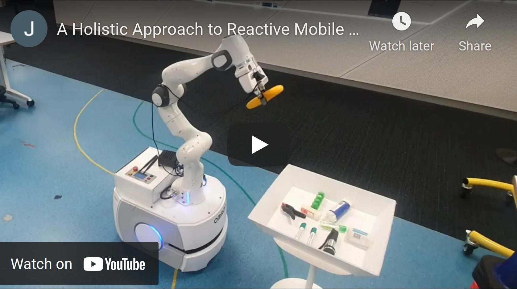
J. Haviland, N. Sünderhauf and P. Corke, "A Holistic Approach to Reactive Mobile Manipulation," in IEEE Robotics and Automation Letters, doi: 10.1109/LRA.2022.3146554. In the video, the robot is controlled using the Robotics toolbox for Python and features a recording from the Swift Simulator.
[Arxiv Paper] [IEEE Xplore] [Project Website] [Video] [Code Example]
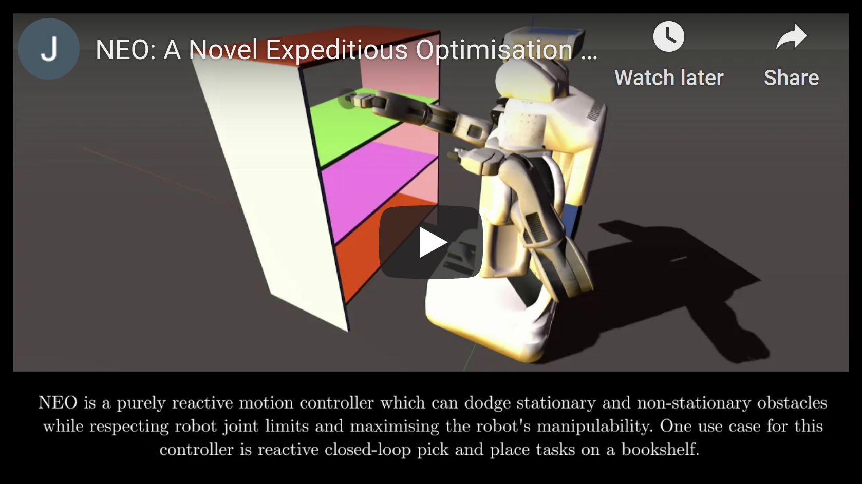
J. Haviland and P. Corke, "NEO: A Novel Expeditious Optimisation Algorithm for Reactive Motion Control of Manipulators," in IEEE Robotics and Automation Letters, doi: 10.1109/LRA.2021.3056060. In the video, the robot is controlled using the Robotics toolbox for Python and features a recording from the Swift Simulator.
[Arxiv Paper] [IEEE Xplore] [Project Website] [Video] [Code Example]
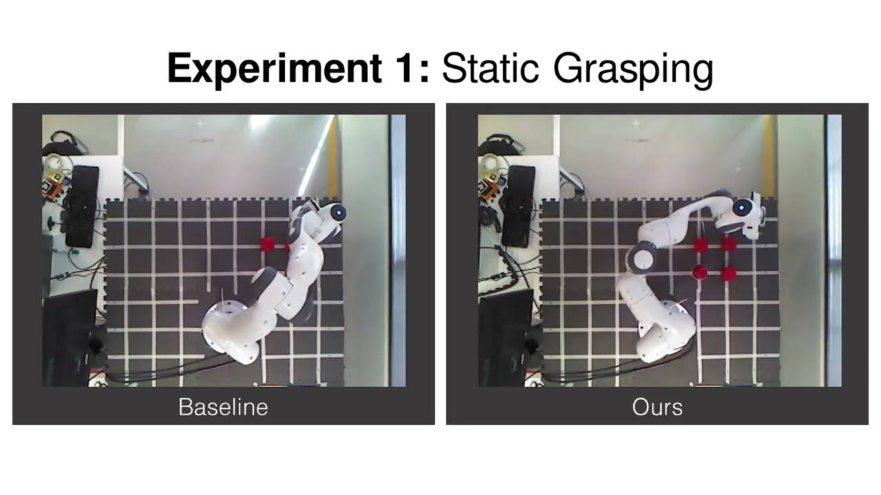
K. He, R. Newbury, T. Tran, J. Haviland, B. Burgess-Limerick, D. Kulić, P. Corke, A. Cosgun, "Visibility Maximization Controller for Robotic Manipulation", in IEEE Robotics and Automation Letters, doi: 10.1109/LRA.2022.3188430. In the video, the robot is controlled using the Robotics toolbox for Python and features a recording from the Swift Simulator.
[Arxiv Paper] [IEEE Xplore] [Project Website] [Video] [Code Example]
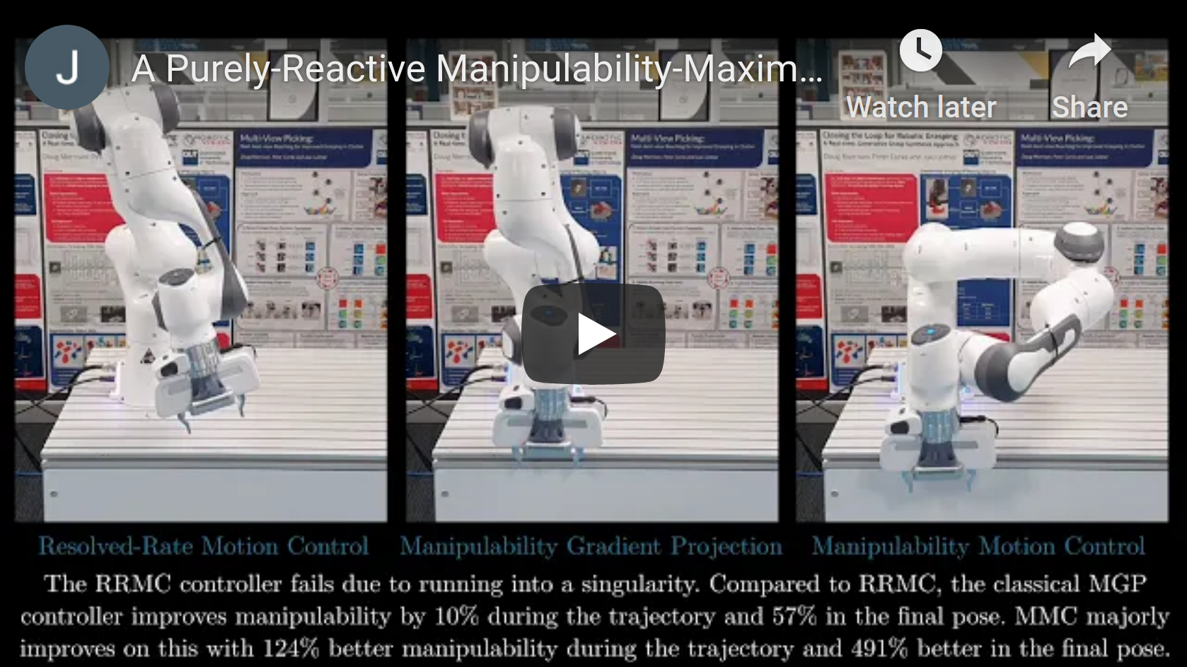
A Purely-Reactive Manipulability-Maximising Motion Controller, J. Haviland and P. Corke. In the video, the robot is controlled using the Robotics toolbox for Python.
[Paper] [Project Website] [Video] [Code Example]
Pyodide is a full CPython distribution compiled to
WebAssembly, which is what lets the "Try it Now" JupyterLite deployment above
run this toolbox entirely client-side, no server required. Each Pyodide
release embeds one specific CPython version, and a wasm wheel is tagged with
the CPython version it was built for (cp312, cp313, ...) -— a wheel only
loads if its tag matches the CPython embedded in the Pyodide runtime actually
running. JupyterLite doesn't bundle Pyodide directly either: the
jupyterlite-pyodide-kernel package pulls in a specific Pyodide version per
its own release, so bumping that one package can silently change which wheel
tag your deployment now needs -— this is the single sharpest edge in this
whole pipeline. This repo's live deployment currently pins
jupyterlite-pyodide-kernel==0.6.1 (see .github/workflows/ci.yml), which
embeds Pyodide 0.27.6 / CPython 3.12 — hence cp312 below.
Also note Pyodide's own version numbering changed in 2026: releases up to
0.29.x used an independent 0.x scheme, but from Pyodide 314.0.0 onward
the version number tracks the embedded CPython version directly (314 =
Python 3.14). "Current" no longer means a 0.x version.
PyPI rejects the pyodide_* platform tag, so Wasm wheels can't be published
there -— instead, every GitHub release attaches ready-built wheels (for each
supported CPython version) as release assets. Download the one matching your
deployment's CPython version, e.g.:
gh release download --repo petercorke/robotics-toolbox-python --pattern '*cp312*pyodide*'This is exactly what ci.yml's docs-build job does to populate the live
"Try it Now" site — most people should do this rather than building locally.
Only needed to test an unreleased change, or to target a different CPython/Pyodide pin than the current release. Uses cibuildwheel's Pyodide platform:
make wheel-pyodideOptionally pin the Pyodide runtime to match a different JupyterLite deployment than this project's own:
PYODIDE_VERSION=0.27.6 make wheel-pyodideThe target writes to dist/ and runs make wheel-pyodide-check, which validates
the wheel filename contains:
cp312-cp312wasm32pyemscripten_<major>_<minor>orpyodide_<major>_<minor>
To inspect the produced artifact path:
ls -1 dist/*wasm32*.whl- Pyodide release notes — confirms what CPython version a given Pyodide tag embeds, including the 2026 versioning-scheme change.
- jupyterlite-pyodide-kernel changelog — the authoritative source for which Pyodide version a given kernel package release bundles.
- cibuildwheel Pyodide platform docs.